Acquiring and stabilizing image sequences
The primary goal of ACE-M2 from a scientific standpoint is to observe the time-evolution of structure and dynamics in samples that may undergo phase separation and/or gelation, in microgravity where sedimentation should not play a role. The stable environment of the ISS and the LMM facilities provide capabilities that are well-suited for this scientific task.
Image acquisition protocol for sample platter 2105
In this fourth run of the ACE-M2 experiment, we have successfully collected about five weeks of continuous data from the six samples in platter 2105 which we expect to undergo phase separation and/or gelation in microgravity (wells d1, e4, e5, f3, f4 and f5).
Each day, for each sample, we collect a full tiling at 10x magnification, to image the entire sample well, at six or more depths. Then, we zoom into a selected area away from the stir bar and bubble, and sample chamber edges, and collect a 2x2 tiling (4 images) at 20x magnification, and a 4x4 tiling (16 images) at 40x. We typically collect all of the images at one magnification, moving through all of the samples, then switching objectives, and collecting images from all six samples at a different magnification, in order to maximize efficiency with operator time.
These image sequences give us both the overview of the entire sample chamber (at lower magnification) and a detailed look at smaller, particular structures (at higher magnification), through the entire sequence of the experiment. This is a powerful combination of capabilities gives a multilengthscale view over time, and will hopefully allow us to understand the physics driving the dynamics of these samples.
Raw ACE-M2 image sequences are not spatially stable
Ideally, we could just load the sample images from the same place over time, and look at the temporal evolution, as we rather commonly do with our microscopes on the ground. Unfortunately, this is simply not possible; every 2D image, nominally from the same position, is slightly shifted every time the image is collected. This could be due to drift, or a lack of stage reproducibility—telling the software to bring the stage back to a nominal x- and y- position should physically move to the same location, +/- only a small distance (a couple of microns, based on the testing on the ground). Unfortunately, we seem to see much greater displacements in the stage on orbit, often tens of microns. Here is an example of the 10 composite tiling from sample 22 (platter 2105, strip B618, well 4), collected at a depth of 80 microns from the cover slip on days 3, 5, 8, 11, 15, 18, 29, 32 and 36:
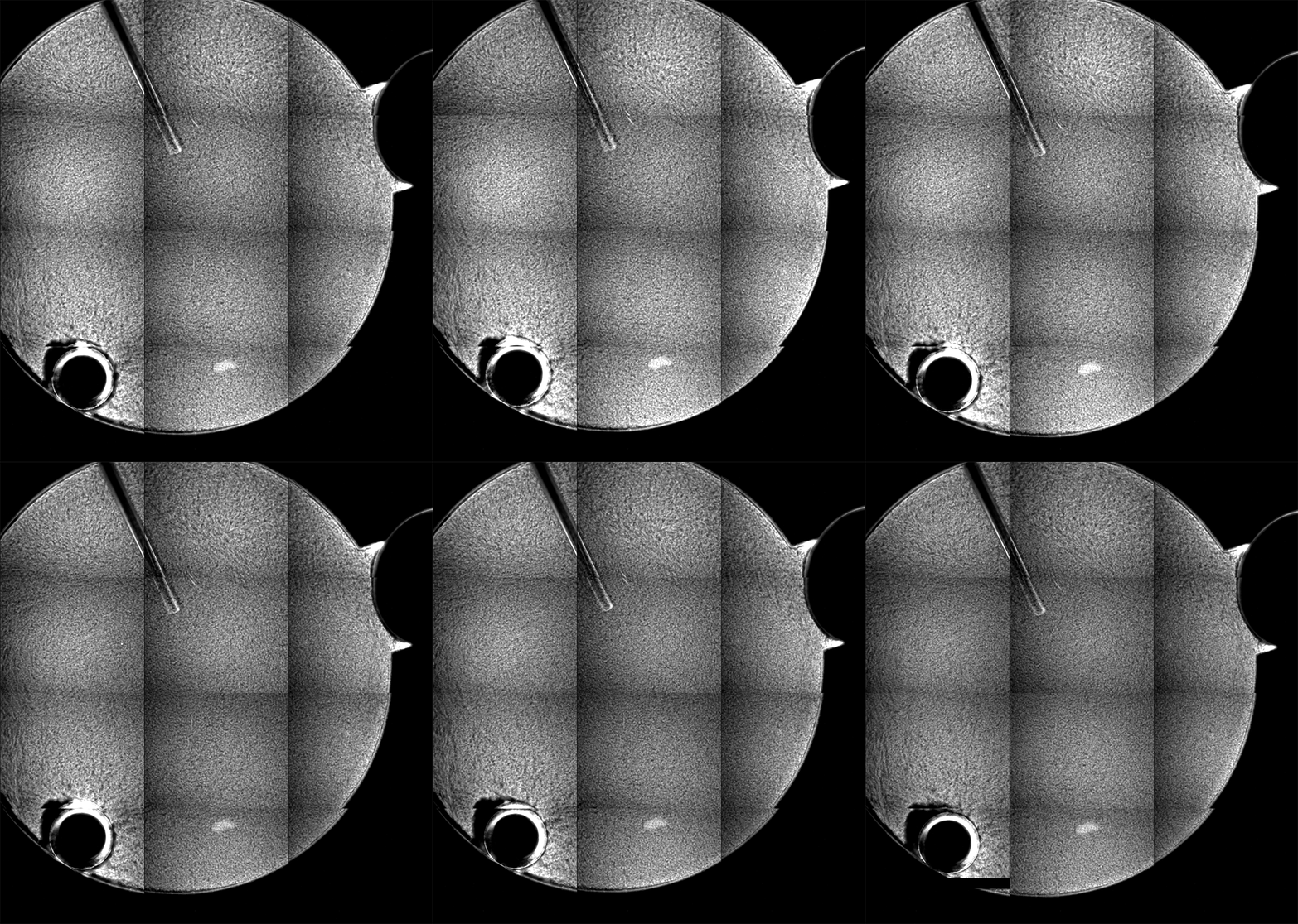
There a delay of 0.1 sec between each image, with a 2-second delay at the end as the movie loops.
The sample chamber is a circle of diameter 2 mm, and is tiled with 3x4 images, so that the shorter edge of each individual image is roughly a half-mm, or 500 microns. The jumps in position from frame to frame are random, and their magnitude is on the order of a tenth of the image edge length, corresponding to a physical distance of around 50 microns. This is about an order of magnitude higher than the nominal stage reproducibility as measured on the ground—and makes the analysis significantly more complicated. Because these jumps are not deterministic, the images must be aligned manually, a very slow, tedious process.
Automated alignment does not work very well
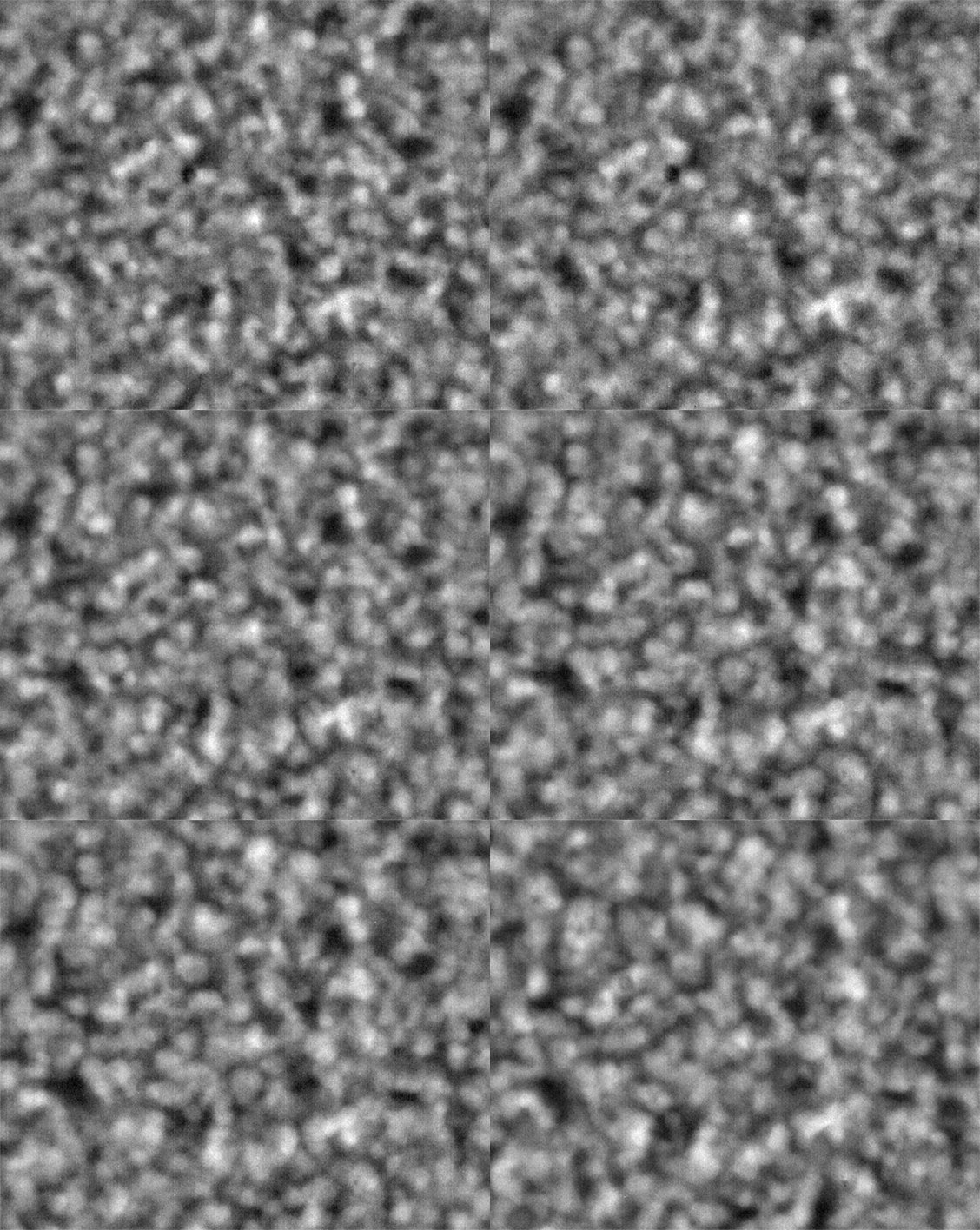
In a previous post, I described the quick-and-dirty method using Photoshop to align composite image sequences in an automated fashion. The problem is that the boundaries of the image move around significantly, due to the large stage displacements, which is not only distracting visually, but prevents the analysis of features near the edge of each image. The skipping is apparent at high magnification, here for sample 21 (platter 2105, strip B618, well 5), collected at a depth of 80 microns from the cover slip on days 4, 5, 8, 11, 15, 18, and 32:
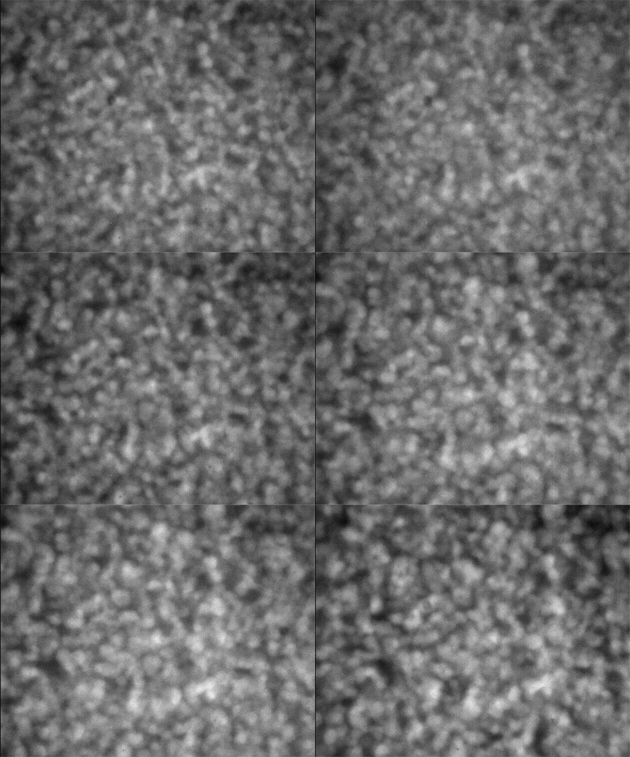

There a delay of 0.5 sec between each image, with a 2-second delay at the end as the movie loops.
Moreover, due to possible fluctuations in lamp intensity, the intensity of images—nominally taken with the same camera settings—is changing, and again in a random, non-deterministic, non-monotonic way.
Image alignment and normalization procedure for ACE-M2 image sequences
The variation in image intensity and position—which fluctuate essentially randomly—requires each individual image to be aligned and adjusted manually. There is no automated procedure to do this is a consistent way. These are grayscale images with features that move and change over time; using stabilization software in Adobe After Effects, for instance, does not remove the motion effectively.
I had a very similar experience with early iterations of the BCAT experiment, so this is not surprising, but does limit the scalability of the experiment in terms of the ability to acquire and manage more data. Nonetheless, I have been able to do the alignment and processing, which are necessary to drawing any scientific conclusions, with a multistep procedure.
Renaming the images
As previously described, every single one of the images in the above sequence has the same file name 00004_00030.tif, and resides in a different directory. Because each file has the same, identical filename, there is no sensible way to import an image sequence into any existing software package without manually renaming each and every file one at a time. Following the previously described image naming convention, the sequence of the images in the above file are of the form p5e5s21_20x_z080_xyd_198.tif, where the last three digits are the numbered day of the year (so the sequence above comprises days 198, 199, 202, 205, 209, 212 and 226).
Aligning and cropping the images
Once renamed, each image is brought into a separate layer in a Photoshop image file, using an included script accessible through the Photoshop CS6 menus: File > scripts > load files into stacks. These are saved as 8-bit grayscale images, which I convert immediately to a 16-bit grayscale file, to preserve as much image information as possible. The alignment procedure basically involves dragging each layer as close as possible to matching the one below it, which is only barely accelerated with the use of a pen tablet and the arrow keys. Rapidly switching layer visibility allows this process to be done correctly, but requires these tedious manual operations. Once the images are aligned, I crop out the areas that do not occur in every image with the crop tool.
Making image intensity consistent
I then filter the images with the despeckle tool, which takes out the pixel noise without affecting much else. In the levels dialog box, I set the black and white points so that there is no clipping, maximizing contrast without losing data. This process works much more effectively in 16-bit grayscale, avoiding posterization.
Next, I remove the intensity profile that causes vignetting (brighter in the center; darker in the corners) with the high pass filter, setting a filter radius of at least 100 pixels, well above the feature size of interest in the images. Then I go back to the levels dialog box and again re-set the white and black points to avoid clipping as a starting point; then I adjust them and the gamma slider to set the average intensity in each image to a grayscale value of 120 (out of 255), and a standard deviation of 30, using the histogram viewer to facilitate interactive adjustment. I then adjust the mapping in the curves dialog box to maintain the same average, but increase the standard deviation to 36, making the images easier to view.
Preparing the animation
Due to noise in the camera’s CCD and general bluriness in the optics, there appears to be no point in presenting the full-size images; therefore, I downsize each image to 50% with a bicubic smoother option in the image size dialog box. Then in the timeline panel, I create frame animiation, and in its menu, make frames from layers and reverse frames. I set the timing, in general, to 0.5 sec per frame, with a 2-second delay at end, before looping (an infinite number of times). Then I export with the save for web command as an animated .gif file, as well as individual frames as .png files.
The resulting final image removes the fluctuations in spatial position and intensity, making the evolution of the sample structure far clearer:
